 |
 |
|
||
|
|
||||

|
Political Calculus SIAM News, June 10, 2001
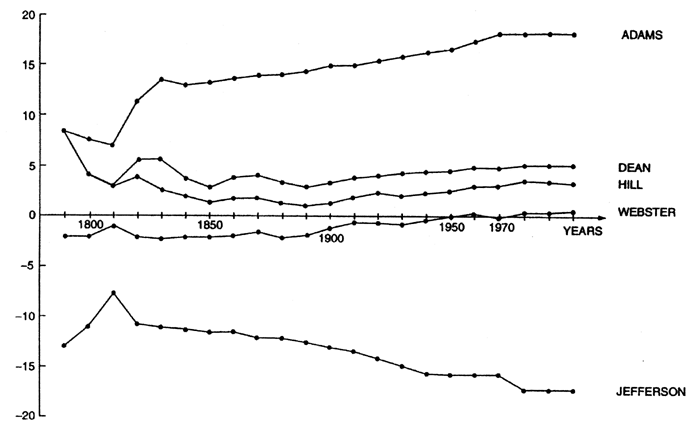
Every ten years, an algorithmic drama plays out in Washington, DC, when official census numbers are fed into a formula that determines the number of seats in the House of Representatives that will be given to each of the 50 states. How many people actually know how the formula works, or where it came from? And is the algorithm fair? Peyton Young, a professor of economics at Johns Hopkins University and a senior fellow at the Brookings Institution, addressed these questions in a session on the mathematics of congressional and other apportionments at the annual meeting of the American Association for the Advancement of Science, held February 15–20, in San Francisco. The formula, which has been in use since 1941, involves the geometric mean. And according to Young, it’s not fair, being biased toward small states. He advocates a return to an earlier system, one devised in 1832 by the statesman Daniel Webster. In a new, updated edition* of their 1982 book Fair Representation: Meeting the Ideal of One Man, One Vote, Young and co-author Michel Balinski (of the Ecole Polytechnique, in Paris) argue that Webster’s method is essentially the only unbiased way to apportion seats in Congress. Rounding Rules Ideally, each member of the House would represent exactly the same number of people as every other member. Offhand, it might seem that the way to come closest to that ideal would be simply to compute each state’s fraction of the total population, multiply by 435 (the total number of seats in the House today), and then round up or down as appropriate to make the total assignment sum to 435. Indeed, that’s the essence of what’s called the Hamilton method, after Alexander Hamilton. In the Hamilton method, the largest fractional parts are rounded up until the total of 435 is reached, and all the others are rounded down. This method was adopted in 1852, when the House was about half its current size (see sidebar), and was used (more or less) until 1901. But the Hamilton method has some problems. The most notorious is called the “Alabama paradox.” In 1881, Congress asked the chief clerk of the Census Bureau to compute the apportionment of seats for each total House size between 275 and 350. (At the time there were 293 seats.) The clerk found something funny: When the total number of seats went from 299 to 300, Alabama actually lost a seat in Congress, dropping from eight seats to seven. It’s easy to see how this might happen. Suppose there are just three “states,” with populations 44, 44, and 12. If there’s to be a “House” with three seats, the quotas are 1.32, 1.32, and .36, so each state gets one representative. But expanding to four seats makes the quotas 1.76, 1.76, and .48, which, by Hamilton’s method, would make the apportionment 2, 2, and 0. (The Constitution, of course, requires that each state have at least one representative. In the actual Alabama paradox of 1880, an increase from 299 to 300 would have benefited Texas and Illinois at the expense of the Yellowhammer State.) The Alabama paradox and another, called the “population paradox,” in which a state loses seats even though its fraction of the nation’s population increases, were denounced—and occasionally exploited—by politicians. In 1901, for example, the chair of the House Select Committee on the 12th census, who had political reasons to dislike Colorado, noticed that the Centennial State would get three seats for any House size between 350 and 400, with the sole exception of 357, which gave Colorado just two seats. He promptly proposed a House size of 357 seats. Fortunately, these and other paradoxes can be avoided by using what are now called “divisor methods.” The first such method was proposed by Thomas Jefferson. In Jefferson’s method, the states’ fractions are simultaneously multiplied by a number slightly greater than 435, after which all the results are rounded down. The multiplier is the key: It must be picked so that the down-rounded numbers sum to 435. There’s a minor mathematical miracle here, in that although there’s a range of possible multipliers, they all give the same apportionment. Jefferson’s method, though, is biased toward large states. In the extreme, it gives no representation to very small states. (The Hamilton method does this too. In either case, an extra provision gives each state at least one seat in the House of Representatives.) Jefferson, of course, came from the largest state of his day. In 1832, ex-president John Quincy Adams proposed a simple variant: Multiply by a number slightly less than 435 and round all the fractions up. This guarantees that everyone is represented, but it’s biased toward small states. According to Webster At around the same time, Daniel Webster suggested splitting the difference: Multiply by an appropriate number near 435 and round fractions to the nearest integer. Webster’s method was adopted in 1842, replaced by Hamilton’s method in 1852, readopted in 1901 (partly in response to the Colorado ruse), and used until 1941. (The history of congressional apportionment is actually quite a bit more byzantine, because the size of the House changed—increasing for the most part, but occasionally shrinking—from 105 seats in 1792 to its current, and seemingly God-given, size of 435 in 1913. The official adoption of Hamilton’s method in 1852, for example, was paired with an increase in the number of seats from 223 to 234. The latter number was chosen in part because the two methods—Hamilton’s and Webster’s—happened to give the same apportionment for the census of 1850. This kind of tinkering, and far worse, complicates any discussion of the history of apportionment methods. But for the last 60 years, at least, things have settled down into a fairly set routine. In recent decades the fights have all been about the numbers that are fed into the apportionment algorithm, not about the algorithm itself.) The 1941 successor to Webster’s method was invented in 1911 by Joseph Hill, a statistician at the Census Bureau, and later refined by Harvard mathematician Edward V. Huntington. It still multiplies the states’ fractions by a number near 435, but its rounding rule is more complicated. For numbers between n and n + 1 (n being an integer), the rounding threshold is the geometric mean, (n (n + 1))1/2. Thus, for example, 1.45 is rounded up to 2 because (1 x 2)1/2 = 1.41 . . . , whereas 52.45 is rounded down because (52 x 53)1/2 = 52.49. . . . The argument in favor of Hill’s method is that, among divisor methods (the only methods that avoid the Alabama and population paradoxes), it minimizes the relative differences among the sizes of representatives’ constituencies. For example, according to the 2000 census, North Carolina’s 8,067,673 people get 13 representatives by Hill’s method, or 620,590 North Carolinians per representative, whereas Utah’s 2,236,714 people warrant three representatives, or 745,571 people per representative— a relative difference of approximately 20.14%. If you swapped a seat, giving North Carolina 12 and Utah four, the numbers would be 672,306 and 559,179, respectively, for a relative difference of 20.23%—even though the absolute difference has decreased (from 124,981 to 113,127)! The method was advocated in a 1929 report from the National Academy of Sciences. It was pegged again as the best method in 1948, in an NAS report signed by the eminent mathematicians Luther Eisenhart, Marston Morse, and John von Neumann. The real reason it was adopted, though, was a purely political calculation: In 1941, the switch from Webster to Hill moved a seat from the swing state of Michigan to the Democratic stronghold of Arkansas. Time for a Change But Hill’s method is biased, Young says. The source of the bias is in the variable rounding: Smaller states have a lower threshold for rounding up. The net effect, he says, is that, over time, small states wind up with 3–4% more representation per capita than the large states.
*Brookings Institution Press, 2001.
|