Fourier/Harmonic Analysis-An Example with Tides
The goal of this section is to provide a concrete example of the Fourier transform and the spectrum of a signal. We will show how the transform data can be used to both understand and exploit the periodic, sinusoidal content of a signal. Specifically, we will look at the problem of predicting the tides by focusing on data collected at the southern end of Manhattan.
|
Figure 4 The star on the charlet shows
the position of the tidal measurement station which collected the data
for this example. This southern part of Manhattan is called The Battery.
Image courtesy of the National Oceanic and Atmospheric Administration
(NOAA), U.S. Department of Commerce |
 |
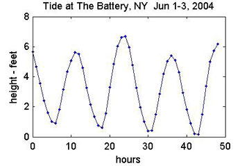
Figure 5 Height of tide as measured at The Battery
- the southern end of Manhattan. The measurements were taken at one
hour intervals. The graphs shows the normal semidiurnal tide pattern,
with one tide cycle taking about 12 hours.
(image courtesy of
NOAA)
|
We learn in our basic science course that the rise and fall of the ocean tides is cause by the gravitational pull of the moon and the sun, interacting with the rotation of the earth, with (generally) about two high tides and two low tides each day (two full cycles).
In 1867, William Thompson (Lord Kelvin) proposed a method for predicting
tides that represented the height of tide based as a sum of sinusoids. Choosing
the appropriate terms to use in that representation is equivalent to identifying
the peaks in amplitude of the Fourier transform. Let h(t) be
the height of tide, measured at some reference point. Since we are interested
in understanding the oscillatory motion, we subtract off the mean height
of tide to find signal
x(t) = h(t) — havg (3)
Then we can compute the associated Fourier transform x(f).
(In fact, because our computation is based on data, we have to use discrete
techniques. We will describe those techniques in the section on The Discrete
Fourier Transform (DFT).) In the context of tides, the input variable
(frequency) is usually measured in degrees per hour (deg/hr) which gives
an angular speed, usually just called speed. Note that a speed of 15 (deg)
would be equivalent to 360 (deg/day) or one cycle per day.
Using data from the National
Oceanic and Atmospheric Administration (NOAA), we selected about 44 months worth of hourly readings and found the resulted Fourier transform data, shown in Figure 6. In the upper panel, we plot amplitude vs. speed over a wide range. The larger the peak, the more significant that frequency is to the overall signal. The peaks near 30 deg/hr are reflecting that the tide has two cycles per day. The peaks near 15 deg/hr are associated with once per day, which results in one of the two high tides during the day being significantly higher than the other.
|
Figure 6 Fourier Transform of tidal data from The Battery - Amplitude vs. Speed. (Upper) For speeds 0-100. The higher the amplitude, the more significant the contribution to the tides. (Lower) Zoomed to speeds near 30 (deg/hour).
(image courtesy of NOAA) |
Near 30 deg/hr, we actually see three peaks, better indicated
on the zoomed in picture of the lower graph. The peak at 30.0 (labeled S2)
is associated with the solar (S) affect on the twice-daily tide (hence the
subscript 2). However, the major peak, labeled M2 is
from the moon, which has the largest effect
on tides. Because the moon is moving relative to the earth, the earth has
to turn a little bit extra to catch up to the moon’s position, which
takes about 24.84 hours (vice 24 hours for the sun), giving a smaller speed
of about 28.98 deg/hr. Because the moon’s
orbit is an ellipse (almost) with the earth at one focus, the moon is not
always at a constant distance from the earth. The N2 component accounts for
this effect.
To predict the tides, NOAA uses the 37 most significant frequencies
from the Fourier analysis, all of which are associated with these astronomical
effects. The speeds (frequencies) of these effects are essentially the same
everywhere, because the relative motions of the earth, moon, and sun are unchanging.
However, location to location, the amplitudes and phases of each must be
determined to be able to compute a predicted tide. That predicted tide is
like doing the Inverse Fourier Transform (IFT), but only approximately, since
only 37 sinusoidal terms are used. To perform that computation, we really
need a computer. Before the advent of the digital computer, this was accomplished
using a mechanical computer. The machine build to do the tidal problem is
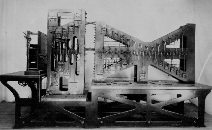
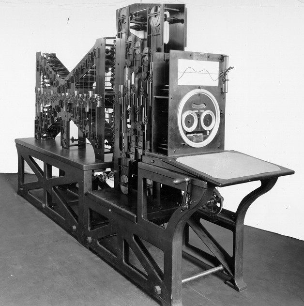
called the Tide Prediction Machine (TPM). From 1910 to 1965, the United States
used Tide Predicting Machine Number 2, a 2,500 pound computer that used pulleys
and gears to compute the sum of the sinusoidal terms, and was also able to
determine the times of highs and lows, and drew a graph of the predicted
tides.
 |
Figure 7 Tide Prediction Machine 2
(Photo courtesy of NOAA) |
 |
Figure 8 TPM Number 2. Note the graph being mechanically drawn.
(Photo courtesy of NOAA) |
Most of the information on the history of harmonic methods for predicting the tides is taken from the NOAA website, a great resource for additional information. For a detailed description, the interested reader can peruse
UNDERSTANDING TIDES, by Steacy Dopp Hicks, Physical Oceanographer


